Keeping it Tidy

Workshop details

Intro 👋
Coding along 💻
Workshop materials ⬇️
Questions ❓

Why R?

R is an open-source (free!) scripting language for working with data

Wonderfully efficient and ✨reproducible✨

Getting R

You need the R language

And also an IDE (I recommend RStudio)

Both are free, helpful installation guide here

Using R

You use R via packages

…which contain functions

…which are just verbs

mutate(), filter(), summarize()

function(argument)

Why the tidyverse?

The tidyverse

An opinionated set of packages that work together and are designed for common data science tasks

Why the tidyverse?

The tidyverse

An opinionated set of packages that work together and are designed for common data science tasks

tidy data!

Why the tidyverse?

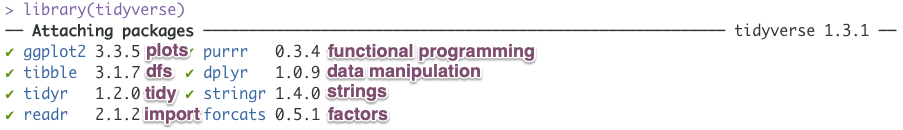
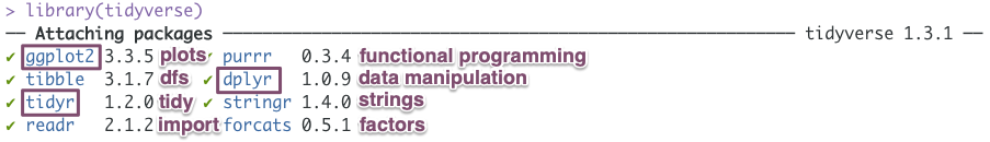
library(tidyverse) The packages loaded with the tidyverse: ggplot2, tibble, tidyr, readr, purrr, dplyr, stringr, forcats

Why the tidyverse?

library(tidyverse) The packages loaded with the tidyverse: ggplot2, tibble, tidyr, readr, purrr, dplyr, stringr, forcats

tidyverse_packages() List of other optional tidyverse packages, including broom, rvest

Common `dplyr` verbs

filter() keeps or discards rows (aka observations)

select() keeps or discards columns (aka variables)

arrange() sorts data set by certain variable(s)

count() tallies data set by certain variable(s)

mutate() creates new variables

summarize() aggregates data

[

these two can be modified by group_by()

Common operators

<- is the assignment operator (think “save as”)

shortcut: option -

|> is the pipe to chain operations together (think recipe instructions)

shortcut: cmd shift m

what about %>%? tidyverse-specific pipe, fine to use!

Today’s data

courtesy of #TidyTuesday

data is from the American Kennel Club

library(tidyverse)
breed_rank <- read_csv("https://raw.githubusercontent.com/meghall06/rladiesparis/master/breed_rank.csv")
breed_traits <- read_csv("https://raw.githubusercontent.com/meghall06/rladiesparis/master/breed_traits.csv")

Today’s data

breed_rank

Breed	2013 Rank	2014 Rank	2015 Rank	2016 Rank	2017 Rank	2018 Rank	2019 Rank	2020 Rank
Retrievers (Labrador)	1	1	1	1	1	1	1	1
French Bulldogs	11	9	6	6	4	4	4	2
German Shepherd Dogs	2	2	2	2	2	2	2	3
Retrievers (Golden)	3	3	3	3	3	3	3	4

Today’s data

breed_traits

Breed	Affectionate With Family	Good With Young Children	Good With Other Dogs	Shedding Level
Retrievers (Labrador)	5	5	5	4
French Bulldogs	5	5	4	3
German Shepherd Dogs	5	5	3	4
Retrievers (Golden)	5	5	5	4

Today’s data

per the tidyverse style guide variable names should use snake case

otherwise variables need to be referred to within `back ticks`

library(janitor)

breed_traits <- breed_traits |> 
  janitor::clean_names()

breed	affectionate_with_family	good_with_young_children
Retrievers (Labrador)	5	5
French Bulldogs	5	5

Today’s data

affectionate_with_family	openness_to_strangers
good_with_young_children	playfulness_level
good_with_other_dogs	watchdog_protective_nature
shedding_level	adaptability_level
coat_grooming_frequency	trainability_level
drooling_level	energy_level
coat_type	barking_level
coat_length	mental_stimulation_needs

Today’s data

affectionate_with_family	openness_to_strangers
good_with_young_children	playfulness_level
good_with_other_dogs	watchdog_protective_nature
shedding_level	adaptability_level
coat_grooming_frequency	trainability_level
drooling_level	energy_level
coat_type	barking_level
coat_length	mental_stimulation_needs

let’s investigate some tidy (and untidy) dogs!

Data verification

use View(breed_traits) to look 👀 at your data

also useful: count()

breed_traits |> 
  count(shedding_level)

shedding_level	n
0	1
1	27
2	41
3	109
4	16
5	1

Data verification

use View(breed_traits) to look 👀 at your data

also useful: count()

breed_traits |> 
  count(shedding_level)

shedding_level	n
0	1
1	27
2	41
3	109
4	16
5	1

Data verification

breed_traits |> 
  filter(shedding_level == 0) |> 
  select(breed, shedding_level, coat_grooming_frequency, 
         drooling_level)

breed	shedding_level	coat_grooming_frequency	drooling_level
Plott Hounds	0	0	0

A cute Plott Hound lounging on the grass

breed_traits <- breed_traits |> 
  filter(shedding_level != 0)

breed_traits |> 
  count(shedding_level)

shedding_level	n
1	27
2	41
3	109
4	16
5	1

A new variable with `mutate()`

untidy_scores <- breed_traits |> 
  mutate(untidy_score = shedding_level + 
           coat_grooming_frequency + drooling_level) |> 
  select(breed, untidy_score)

breed	untidy_score
Retrievers (Labrador)	8
French Bulldogs	7
German Shepherd Dogs	8
Retrievers (Golden)	8
Bulldogs	9

Sorting with `arrange()`

untidy_scores |> 
  arrange(untidy_score)

breed	untidy_score
American Hairless Terriers	3
Xoloitzcuintli	3
Cirnechi dell Etna	3
Chihuahuas	4
Whippets	4
Chinese Crested	4

Sorting with `arrange()`

untidy_scores |> 
  arrange(desc(untidy_score))

breed	untidy_score
Bernese Mountain Dogs	11
Leonbergers	11
Newfoundlands	10
Bloodhounds	10
St. Bernards	10
Old English Sheepdogs	10

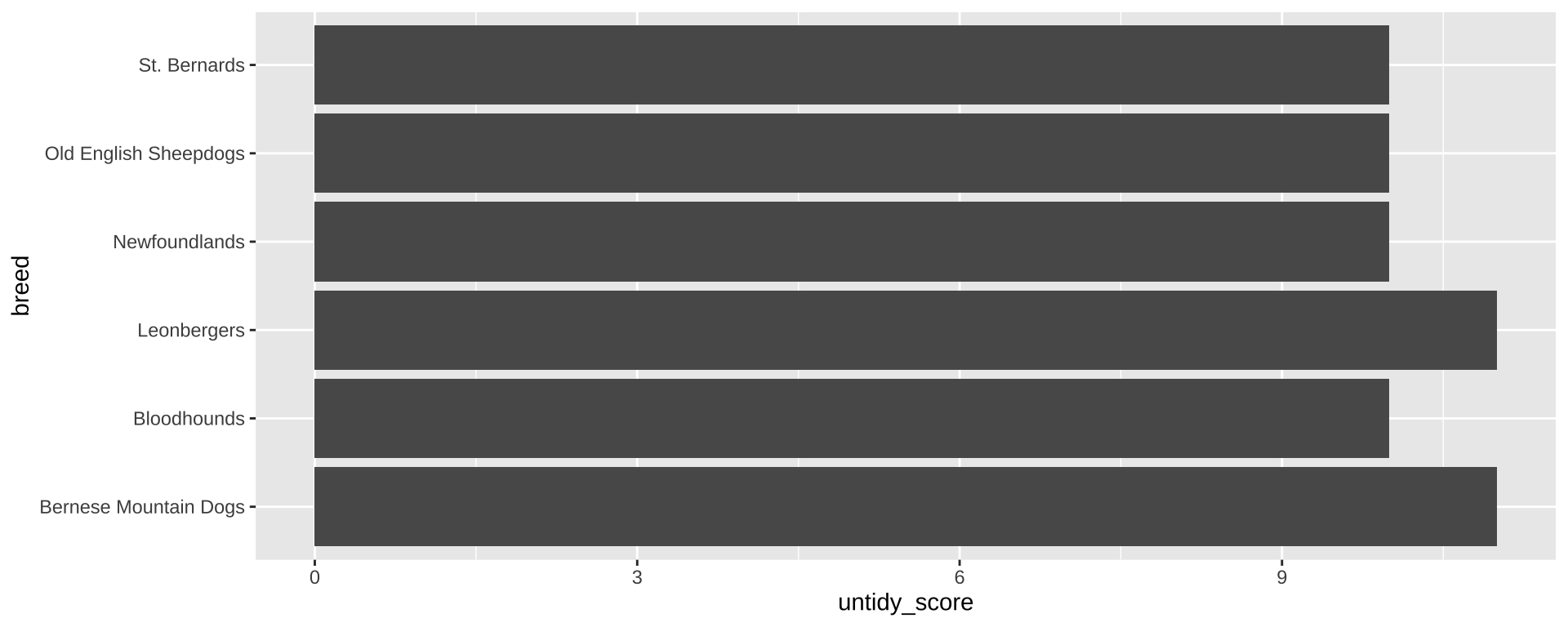
Bar chart

can we plot the scores of the untidiest dogs?

untidy_dogs <- untidy_scores |> 
  slice_max(untidy_score, n = 6, with_ties = FALSE)

breed	untidy_score
Bernese Mountain Dogs	11
Leonbergers	11
Newfoundlands	10
Bloodhounds	10
St. Bernards	10
Old English Sheepdogs	10

untidy_dogs |> 
  ggplot(aes(x = untidy_score, y = breed)) +
  geom_bar(stat = "identity")

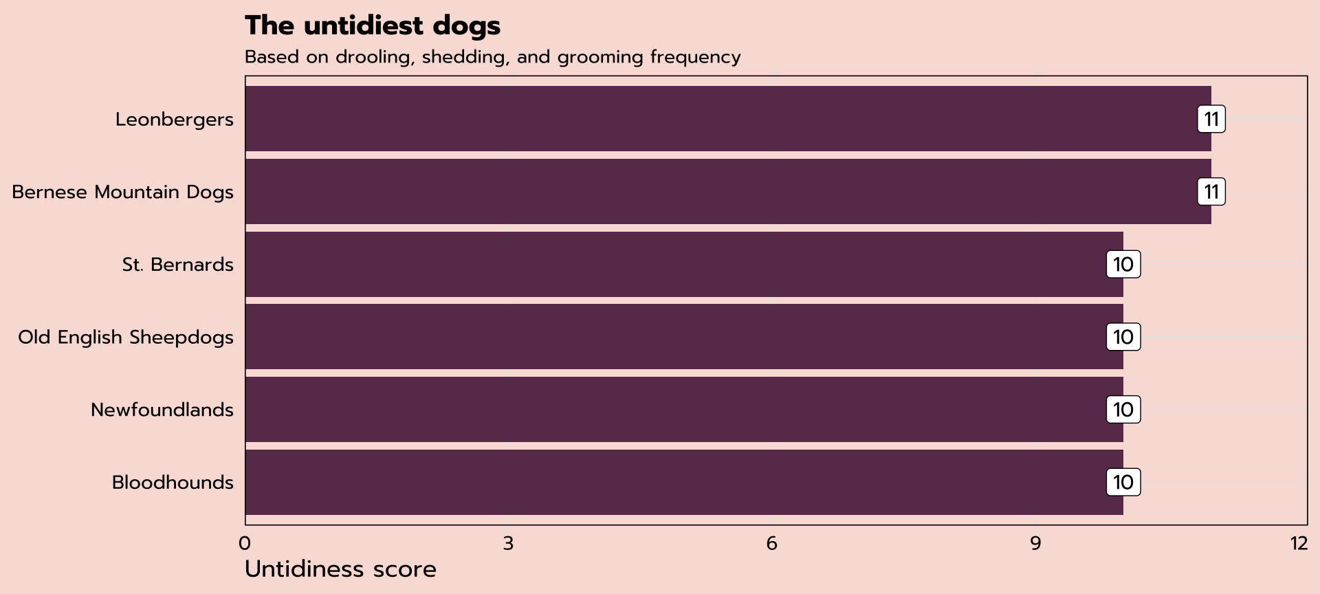
expand for full code

untidy_dogs |> 
  ggplot(aes(x = untidy_score, y = reorder(breed, untidy_score), 
             label = untidy_score)) +
  geom_bar(stat = "identity", fill = "#6A395B") +
  geom_label(family = "prompt") +
  scale_x_continuous(expand = expansion(mult = c(0, 0.1))) +
  labs(title = "The untidiest dogs",
       subtitle = "Based on drooling, shedding, and grooming frequency",
       x = "Untidiness score", y = NULL) +
  theme_tidy_dog()

Tidy data

Bernese Mountain Dogs are the untidiest of all—how does their popularity rank change over time?

Breed	2013 Rank	2014 Rank	2015 Rank	2016 Rank	2017 Rank	2018 Rank	2019 Rank	2020 Rank
Bernese Mountain Dogs	32	32	29	27	25	22	23	22

ggplot(aes(x = ??, y = ??))

Tidy data

There are three interrelated rules which make a dataset tidy:
1. Each variable must have its own column.
2. Each observation must have its own row.
3. Each value must have its own cell.
- R for Data Science

Breed	2013 Rank	2014 Rank	2015 Rank	2016 Rank	2017 Rank	2018 Rank	2019 Rank	2020 Rank
Bernese Mountain Dogs	32	32	29	27	25	22	23	22

Tidy data

There are three interrelated rules which make a dataset tidy:
1. Each variable must have its own column.
2. Each observation must have its own row.
3. Each value must have its own cell.
- R for Data Science

Breed	2013 Rank	2014 Rank	2015 Rank	2016 Rank	2017 Rank	2018 Rank	2019 Rank	2020 Rank
Bernese Mountain Dogs	32	32	29	27	25	22	23	22

how does this violate the tidy data rules?

`pivot_longer()` for tidy data

ranks_pivoted <- breed_rank |> 
  pivot_longer(`2013 Rank`:`2020 Rank`,
               names_to = "year",
               values_to = "rank")

Breed	year	rank
Bernese Mountain Dogs	2013 Rank	32
Bernese Mountain Dogs	2014 Rank	32
Bernese Mountain Dogs	2015 Rank	29
Bernese Mountain Dogs	2016 Rank	27
Bernese Mountain Dogs	2017 Rank	25
Bernese Mountain Dogs	2018 Rank	22
Bernese Mountain Dogs	2019 Rank	23
Bernese Mountain Dogs	2020 Rank	22

`pivot_longer()` for tidy data

ranks_pivoted <- ranks_pivoted |> 
  rename(breed = Breed) |> 
  mutate(year = parse_number(year))

breed	year	rank
Bernese Mountain Dogs	2013	32
Bernese Mountain Dogs	2014	32
Bernese Mountain Dogs	2015	29
Bernese Mountain Dogs	2016	27
Bernese Mountain Dogs	2017	25
Bernese Mountain Dogs	2018	22
Bernese Mountain Dogs	2019	23
Bernese Mountain Dogs	2020	22

`pivot_longer()` for tidy data

Bernese Mountain Dogs are the untidiest of all—how does their popularity rank change over time?

breed	year	rank
Bernese Mountain Dogs	2013	32
Bernese Mountain Dogs	2014	32
Bernese Mountain Dogs	2015	29
Bernese Mountain Dogs	2016	27
Bernese Mountain Dogs	2017	25

ggplot(aes(x = year, y = rank))

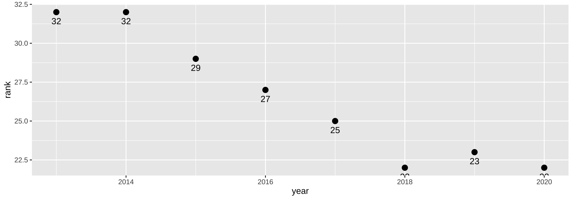
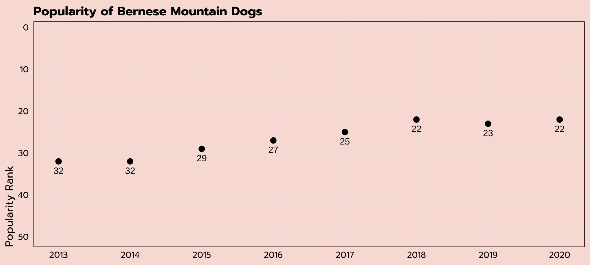
Dot plot

Basic
Custom

ranks_pivoted |> 
  filter(str_detect(breed, "Bernese")) |> 
  ggplot(aes(x = year, y = rank, label = rank)) +
  geom_point(size = 3) +
  geom_text(vjust = 2)

expand for full code

ranks_pivoted |> 
  filter(str_detect(breed, "Bernese")) |> 
  ggplot(aes(x = year, y = rank, label = rank)) +
  geom_point(size = 3) +
  geom_text(vjust = 2) +
  scale_y_reverse(limits = c(50, 1)) +
  scale_x_continuous(breaks = seq(2013, 2020, 1)) +
  labs(x = NULL, y = "Popularity Rank",
       title = "Popularity of Bernese Mountain Dogs") +
  theme_tidy_dog()

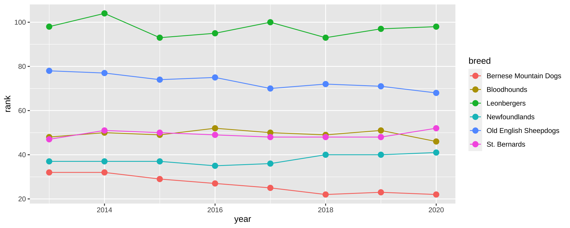
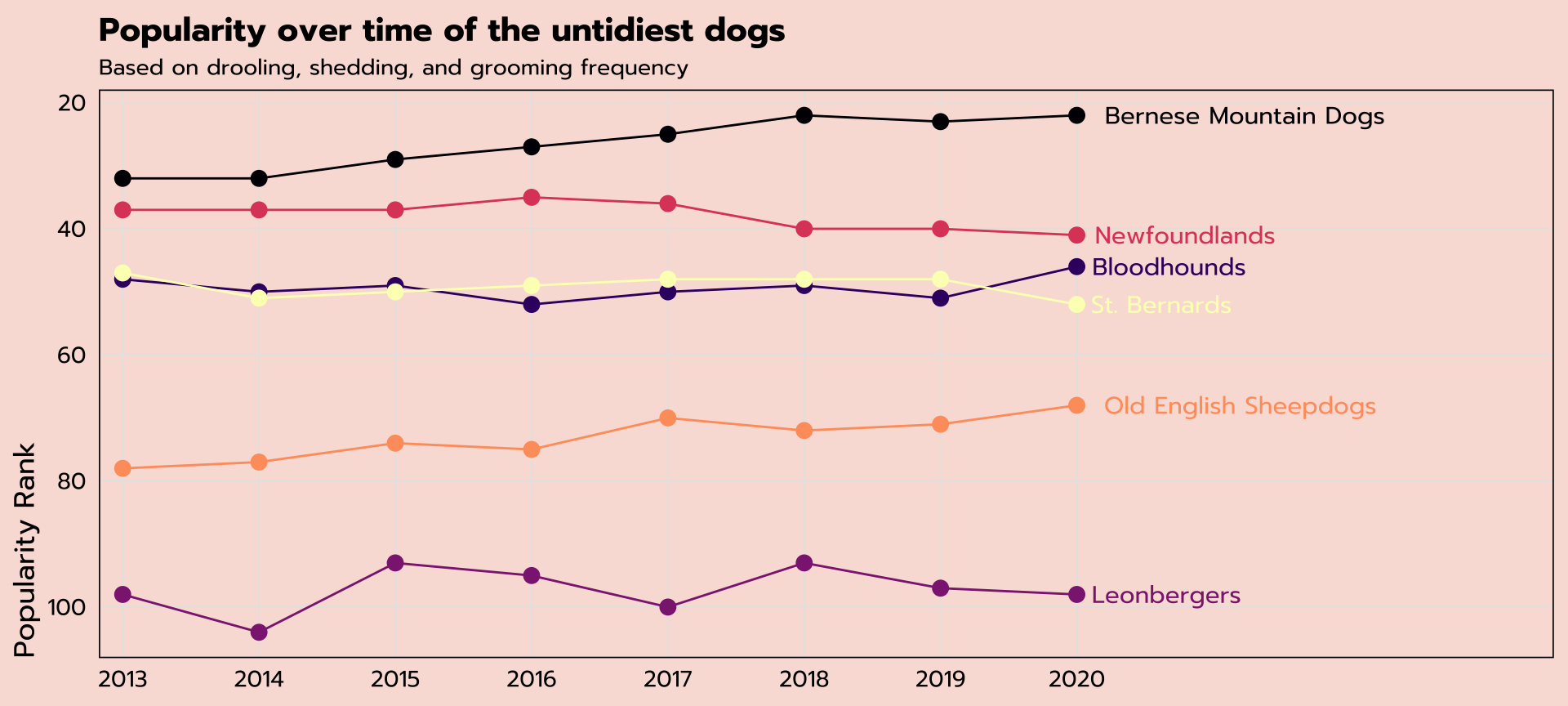
Line graph

can we plot the popularity ranking of the untidiest dogs?

untidy_dogs

breed	untidy_score
Bernese Mountain Dogs	11
Leonbergers	11
Newfoundlands	10
Bloodhounds	10
St. Bernards	10
Old English Sheepdogs	10

ranks_pivoted

breed	year	rank
Retrievers (Labrador)	2013	1
Retrievers (Labrador)	2014	1
Retrievers (Labrador)	2015	1
Retrievers (Labrador)	2016	1
Retrievers (Labrador)	2017	1
Retrievers (Labrador)	2018	1

untidy_popularity <- ranks_pivoted |> 
  filter(breed %in% untidy_dogs$breed)

Line graph

check that this filtered the way we wanted it to!

untidy_popularity |> 
  count(breed)

breed	n
Bernese Mountain Dogs	8
Bloodhounds	8
Leonbergers	8
Newfoundlands	8
Old English Sheepdogs	8
St. Bernards	8

Line graph

Basic
Custom

untidy_popularity |> 
  ggplot(aes(x = year, y = rank, group = breed, color = breed)) +
  geom_line() +
  geom_point(size = 3)

expand for full code

untidy_popularity |> 
  mutate(label = ifelse(year == 2020, breed, NA)) |> 
  ggplot(aes(x = year, y = rank, group = breed, color = breed,
             label = label)) +
  geom_line() +
  geom_point(size = 3) +
  geom_text(hjust = -0.1, family = "prompt") +
  scale_color_viridis_d(option = "A") +
  scale_x_continuous(expand = expansion(mult = c(0.025, 0.5)),
                     breaks = seq(2013, 2020, 1)) +
  scale_y_reverse() +
  labs(title = "Popularity over time of the untidiest dogs",
       subtitle = "Based on drooling, shedding, and grooming frequency",
       x = NULL,
       y = "Popularity Rank") +
  theme_tidy_dog() +
  theme(legend.position = "none")

Relational data: `left_join()`

can we plot the average popularity ranking against the tidy_scores for all dogs?

avg_ranks <- ranks_pivoted |> 
  group_by(breed) |> 
  summarize(avg_rank = mean(rank))

breed	avg_rank
Affenpinschers	147.750
Afghan Hounds	105.875
Airedale Terriers	57.375
Akitas	46.500
Alaskan Malamutes	58.875
American English Coonhounds	169.125
American Eskimo Dogs	118.875
American Foxhounds	185.250
American Hairless Terriers	NA

Relational data: `left_join()`

can we plot the average popularity ranking against the tidy_scores for all dogs?

avg_ranks <- ranks_pivoted |> 
  group_by(breed) |> 
  summarize(avg_rank = mean(rank, na.rm = TRUE))

breed	avg_rank
Affenpinschers	147.750
Afghan Hounds	105.875
Airedale Terriers	57.375
Akitas	46.500
Alaskan Malamutes	58.875
American English Coonhounds	169.125
American Eskimo Dogs	118.875
American Foxhounds	185.250
American Hairless Terriers	129.000

Relational data: `left_join()`

can we plot the average popularity ranking against the tidy_scores for all dogs?

avg_ranks

breed	avg_rank
Affenpinschers	147.750
Afghan Hounds	105.875
Airedale Terriers	57.375
Akitas	46.500
Alaskan Malamutes	58.875

untidy_scores

breed	untidy_score
Retrievers (Labrador)	8
French Bulldogs	7
German Shepherd Dogs	8
Retrievers (Golden)	8
Bulldogs	9

Relational data: `left_join()`

other join types are available, but left_join() is the most common (more info in R4DS)

tidy_and_rank <- avg_ranks |> 
  left_join(untidy_scores, by = "breed")

can specify keys with by = "var"

multiple: by = c("var1","var2")
different names: by = c("var_left" = "var_right")

breed	avg_rank	untidy_score
Affenpinschers	147.750	7
Afghan Hounds	105.875	6

Relational data: `left_join()`

check that this worked the way we wanted it to!

tidy_and_rank |> 
  count(untidy_score)

untidy_score	n
3	3
4	13
5	25
6	43
7	59
8	30
9	11
10	8
11	2
NA	1

Relational data: `left_join()`

tidy_and_rank |> 
  filter(is.na(untidy_score))

breed	avg_rank	untidy_score
Plott Hounds	167	NA

tidy_and_rank <- tidy_and_rank |> 
  filter(!is.na(untidy_score))

untidy_score	n
3	3
4	13
5	25
6	43
7	59
8	30
9	11
10	8
11	2

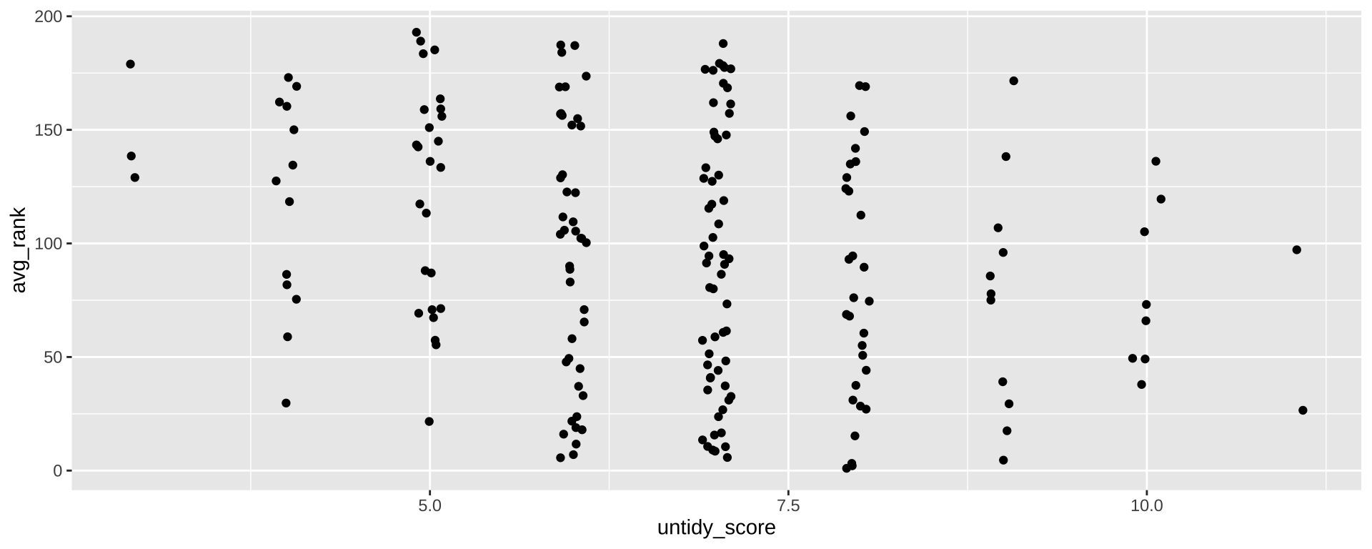
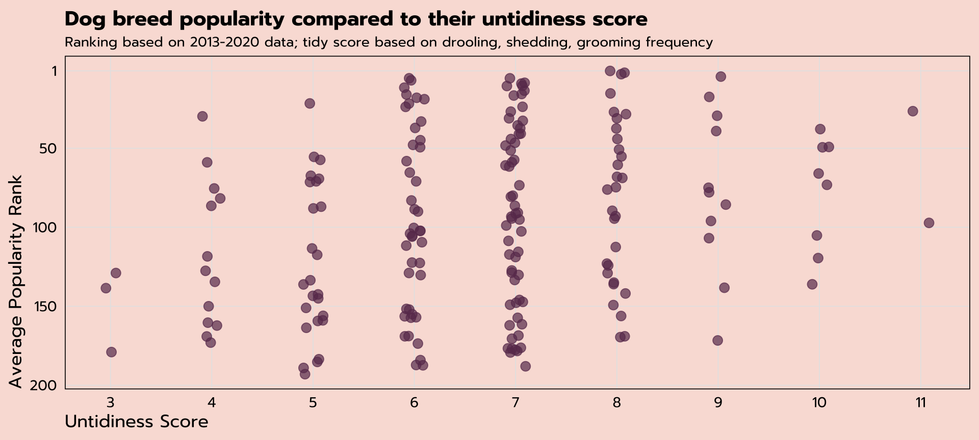
Jitter plot

Basic
Custom

tidy_and_rank |> 
  ggplot(aes(x = untidy_score, y = avg_rank)) +
  geom_jitter(width = 0.1)

expand for full code

tidy_and_rank |>  
  ggplot(aes(x = untidy_score, y = avg_rank)) +
  scale_x_continuous(breaks = seq(3, 11, 1)) +
  geom_jitter(size = 3, width = 0.1, alpha = 0.7, color = "#6A395B") +
  scale_y_reverse(breaks = c(200, 150, 100, 50, 1)) +
  labs(title = "Dog breed popularity compared to their untidiness score",
       subtitle = "Ranking based on 2013-2020 data; tidy score based on drooling, shedding, grooming frequency",
       x = "Untidiness Score",
       y = "Average Popularity Rank") +
  theme_tidy_dog()

`pivot_wider()`

which breeds have had the biggest jump in popularity?

ranks_pivoted

breed	year	rank
Retrievers (Labrador)	2013	1
Retrievers (Labrador)	2014	1
Retrievers (Labrador)	2015	1
Retrievers (Labrador)	2016	1
Retrievers (Labrador)	2017	1
Retrievers (Labrador)	2018	1
Retrievers (Labrador)	2019	1
Retrievers (Labrador)	2020	1
French Bulldogs	2013	11

`pivot_wider()`

which breeds have had the biggest jump in popularity?

ranks_pivoted

breed	year	rank
Retrievers (Labrador)	2013	1
Retrievers (Labrador)	2014	1
Retrievers (Labrador)	2015	1
Retrievers (Labrador)	2016	1
Retrievers (Labrador)	2017	1
Retrievers (Labrador)	2018	1
Retrievers (Labrador)	2019	1
Retrievers (Labrador)	2020	1
French Bulldogs	2013	11

`pivot_wider()`

will all deliver the same results:

filter(year %in% c(2013, 2020))
filter(year == 2013 | year == 2020)
filter(year == min(year) | year == max(year))

most robust option ☝️

`pivot_wider()`

rank_change <- ranks_pivoted |>  
  filter(year == min(year) | year == max(year)) |> 
  pivot_wider(names_from = "year",
              values_from = "rank") |>  
  mutate(change = `2013` - `2020`) |> 
  filter(`2020` <= 50) |>  
  slice_max(change, n = 6)

breed	2013	2020	change
Cane Corso	50	25	25
Belgian Malinois	60	37	23
Spaniels (English Cocker)	62	47	15
Pembroke Welsh Corgis	24	11	13
Border Collies	44	32	12
Bernese Mountain Dogs	32	22	10

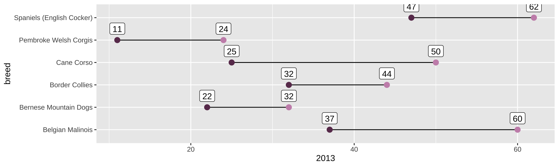
Dumbbell plot

useful plot type for showing change between two points

to be honest: it’s easier to make these with ggalt::geom_dumbbell()

but we can use ggplot2 to learn a) how to combine multiple geoms and b) how inherited aes works

Dumbbell plot

Basic
Custom

rank_change |>  
  ggplot(aes(y = breed)) +
  geom_segment(aes(yend = breed, x = `2013`, xend = `2020`)) +
  geom_point(aes(x = `2013`), color = "#c991b8", size = 3) +
  geom_point(aes(x = `2020`), color = "#6A395B", size = 3) +
  geom_label(aes(x = `2020`, label = `2020`), vjust = -0.5) +
  geom_label(aes(x = `2013`, label = `2013`), vjust = -0.5)

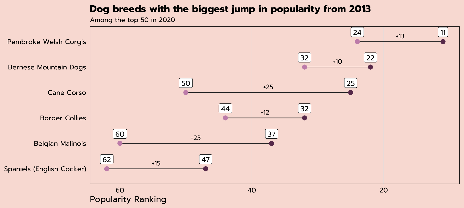
expand for full code

rank_change |>  
  mutate(middle = `2020` + (change / 2)) |>  
  ggplot(aes(y = reorder(breed, -`2020`))) +
  geom_segment(aes(yend = reorder(breed, -`2020`), x = `2013`, xend = `2020`), 
               color = "grey20") +
  geom_point(aes(x = `2013`), color = "#c991b8", size = 3) +
  geom_point(aes(x = `2020`), color = "#6A395B", size = 3) +
  geom_label(aes(x = `2020`, label = `2020`), family = "prompt", vjust = -0.5) +
  geom_label(aes(x = `2013`, label = `2013`), family = "prompt", vjust = -0.5) +
  geom_text(aes(x = middle, label = str_c("+", change)), family = "prompt", 
            vjust = -0.75, size = 3.5) +
  scale_x_reverse() +
  labs(x = "Popularity Ranking",
       y = NULL,
       title = "Dog breeds with the biggest jump in popularity from 2013",
       subtitle = "Among the top 50 in 2020") +
  theme_tidy_dog() +
  theme(panel.grid.major.y = element_blank())

Go forth and code!

Two corgis trotting on a treadmill.

`ggplot` theme

library(showtext)

# Add Google fonts
font_add_google("Prompt", "prompt")

showtext_auto()

theme_tidy_dog <- function () { 
  theme_linedraw(base_size=13, base_family="prompt") %+replace% 
    theme(
      axis.title = element_text(hjust = 0),
      panel.background = element_rect(fill='#F9E0D9', color = NA),
      plot.background = element_rect(fill='#F9E0D9', color=NA),
      legend.background = element_rect(fill="transparent", color=NA),
      legend.key = element_rect(fill="transparent", color=NA),
      axis.ticks = element_blank(),
      panel.grid.major = element_line(color = "grey90", size = 0.3), 
      panel.grid.minor = element_blank(),
      plot.title = element_text(size = 15, hjust = 0, vjust = 0.5, face = "bold", 
                                margin = margin(b = 0.2, unit = "cm")),
      plot.subtitle = element_text(size = 10, hjust = 0, vjust = 0.5, 
                                   margin = margin(b = 0.2, unit = "cm")),
    )
}

Resources

R for Data Science: the ultimate guide

R for Excel users: a very useful workshop

STAT 545: online book on reproducible data analysis

the RStudio Education site

the Learn tidyverse site

Thank you!

MEGHAN HALL
@MeghanMHall
meghall06
meghan.rbind.io
meghanhall6 AT gmail

slides made with Quarto 🎉

Keeping it Tidy

Workshop details

Why R?

Getting R

Using R

Why the tidyverse?

Why the tidyverse?

Why the tidyverse?

Why the tidyverse?

Common dplyr verbs

Common operators

Today’s data

Today’s data

Today’s data

Today’s data

Today’s data

Today’s data

Data verification

Data verification

Data verification

A new variable with mutate()

Sorting with arrange()

Sorting with arrange()

Bar chart

Bar chart

Tidy data

Tidy data

Tidy data

pivot_longer() for tidy data

pivot_longer() for tidy data

pivot_longer() for tidy data

Dot plot

Line graph

Line graph

Line graph

Relational data: left_join()

Relational data: left_join()

Relational data: left_join()

Relational data: left_join()

Relational data: left_join()

Relational data: left_join()

Jitter plot

pivot_wider()

pivot_wider()

pivot_wider()

pivot_wider()

Dumbbell plot

Dumbbell plot

Go forth and code!

ggplot theme

Resources

Common `dplyr` verbs

A new variable with `mutate()`

Sorting with `arrange()`

Sorting with `arrange()`

`pivot_longer()` for tidy data

`pivot_longer()` for tidy data

`pivot_longer()` for tidy data

Relational data: `left_join()`

Relational data: `left_join()`

Relational data: `left_join()`

Relational data: `left_join()`

Relational data: `left_join()`

Relational data: `left_join()`

`pivot_wider()`

`pivot_wider()`

`pivot_wider()`

`pivot_wider()`

`ggplot` theme