Streamlining with R
Meghan Hall
NEAIR
July 12, 2022
Housekeeping
- Intro 👋
- Workshop materials ⬇️
- Break 🕘
- By the end of today ✔️
- Today’s plan 📋
Today’s plan
- What is R? How can it ease the burden of repeated reporting?
- Basic functions for manipulating data
- Using R effectively
- More data manipulation
- Visualizing data
- A peek at advanced topics
What is R?
1 2 3 4 5 6
What is R?
1 2 3 4 5 6
R is an open-source (free!) scripting language for working with data
The benefits of R
1 2 3 4 5 6
My personal Excel nightmare
The magic of R is that it’s reproducible (by someone else or by yourself in six months)
Keeps data separate from code (data preparation steps)
Getting R
1 2 3 4 5 6
You need the R language
And also the software
Navigating RStudio
1 2 3 4 5 6
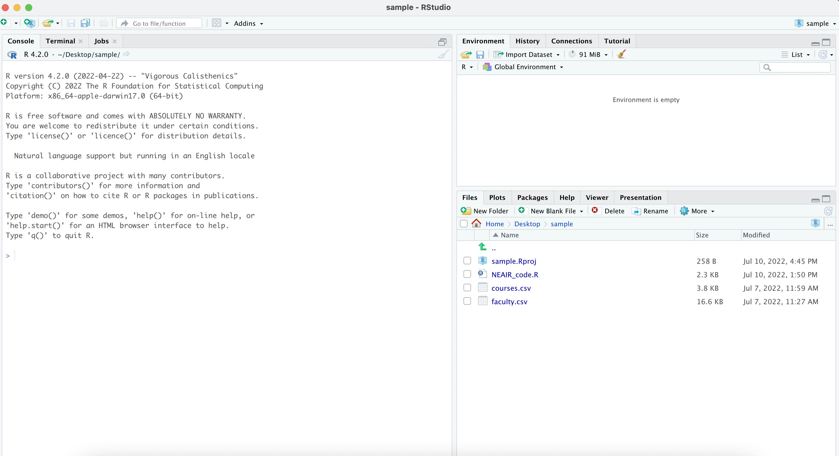
project files are here
imported data shows up here
code can go here
Navigating RStudio
1 2 3 4 5 6
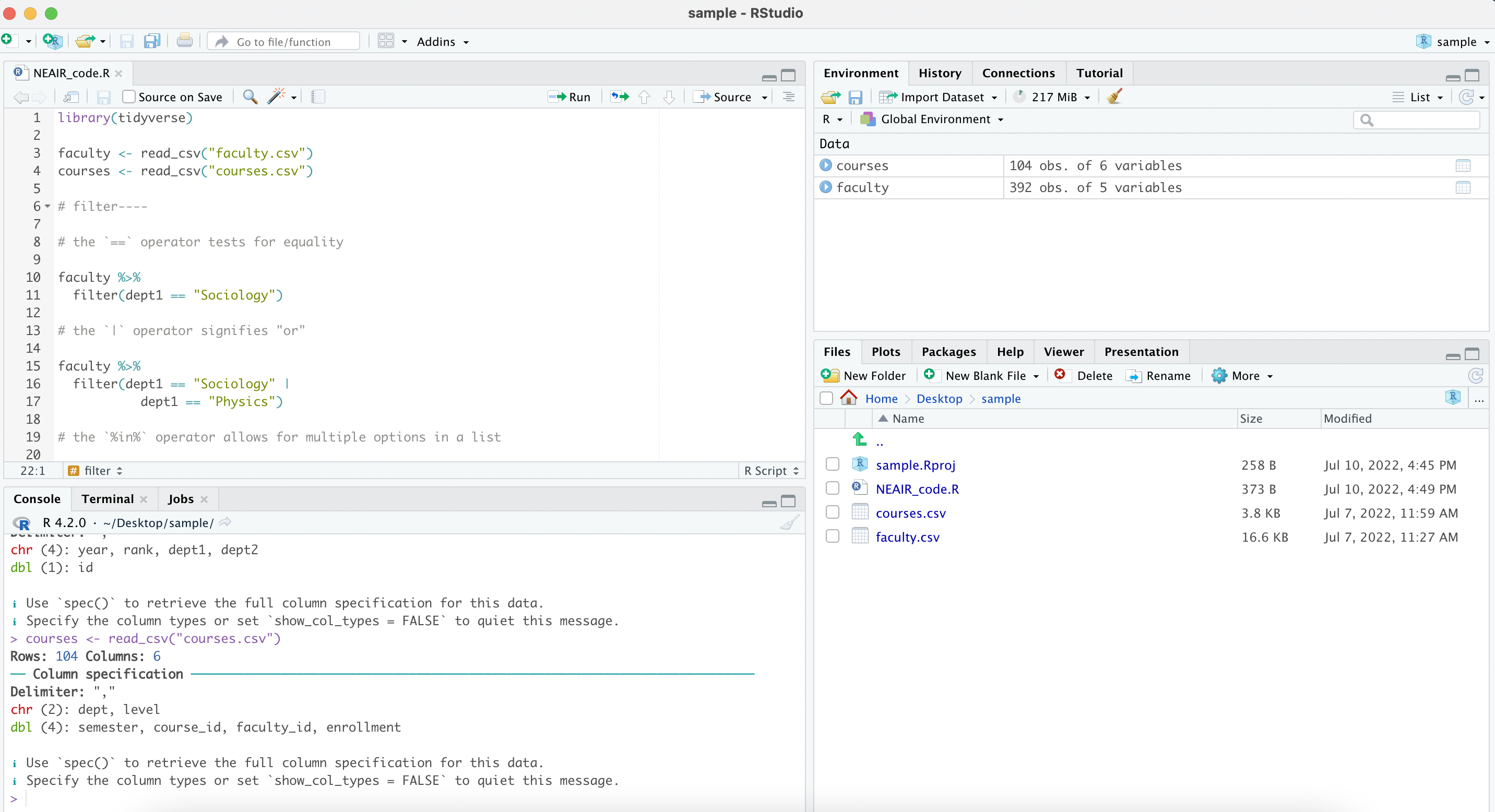
project files are here
imported data shows up here
code can also
go here
Using R
1 2 3 4 5 6
You use R via packages
…which contain functions
…which are just verbs
Today’s data
1 2 3 4 5 6
faculty
| year | id | rank | dept1 | dept2 |
|---|---|---|---|---|
| 2021-22 | 1005 | Lecturer | Chemistry | |
| 2021-22 | 1022 | Professor | Physics | Engineering |
| 2021-22 | 1059 | Professor | Physics | |
| 2021-22 | 1079 | Lecturer | Music | |
| 2021-22 | 1086 | Assistant Professor | Music | |
| 2021-22 | 1095 | Adjunct Instructor | Sociology |
Today’s data
1 2 3 4 5 6
courses
| semester | course_id | faculty_id | dept | enrollment | level |
|---|---|---|---|---|---|
| 20212202 | 10605 | 1772 | Physics | 7 | UG |
| 20212202 | 10605 | 1772 | Physics | 32 | GR |
| 20212202 | 11426 | 1820 | Political Science | 8 | UG |
| 20212202 | 12048 | 1914 | English | 24 | UG |
| 20212202 | 13269 | 1095 | Sociology | 48 | UG |
| 20212202 | 13517 | 1086 | Music | 17 | UG |
Basic data manipulation
1 2 3 4 5 6
Useful operators
1 2 3 4 5 6
<-
“save as”
opt + -
%>%
“and then”
Cmd + shift + m
Common functions
1 2 3 4 5 6
filter keeps or discards rows (aka observations)
select keeps or discards columns (aka variables)
arrange sorts data set by certain variable(s)
count tallies data set by certain variable(s)
mutate creates new variables
group_by/summarize aggregates data (pivot tables!)
str_* functions work easily with text
Syntax of a function
1 2 3 4 5 6
function(data, argument(s))
is the same as
data %>%
function(argument(s))
Filter
1 2 3 4 5 6
filter keeps or discards rows (aka observations)
the == operator tests for equality
| year | id | rank | dept1 | dept2 |
|---|---|---|---|---|
| 2021-22 | 1095 | Adjunct Instructor | Sociology | |
| 2021-22 | 1118 | Assistant Professor | Sociology | |
| 2021-22 | 1161 | Assistant Professor | Sociology | |
| 2021-22 | 1191 | Professor | Sociology | |
| 2021-22 | 1216 | Associate Professor | Sociology | American Studies |
| 2021-22 | 1273 | Assistant Professor | Sociology |
Filter
1 2 3 4 5 6
the | operator signifies “or”
| year | id | rank | dept1 | dept2 |
|---|---|---|---|---|
| 2021-22 | 1022 | Professor | Physics | Engineering |
| 2021-22 | 1059 | Professor | Physics | |
| 2021-22 | 1095 | Adjunct Instructor | Sociology | |
| 2021-22 | 1118 | Assistant Professor | Sociology | |
| 2021-22 | 1161 | Assistant Professor | Sociology | |
| 2021-22 | 1191 | Professor | Sociology |
Filter
1 2 3 4 5 6
the %in% operator allows for multiple options in a list
| year | id | rank | dept1 | dept2 |
|---|---|---|---|---|
| 2021-22 | 1022 | Professor | Physics | Engineering |
| 2021-22 | 1059 | Professor | Physics | |
| 2021-22 | 1079 | Lecturer | Music | |
| 2021-22 | 1086 | Assistant Professor | Music | |
| 2021-22 | 1095 | Adjunct Instructor | Sociology | |
| 2021-22 | 1118 | Assistant Professor | Sociology |
Filter
1 2 3 4 5 6
the & operator combines conditions
| year | id | rank | dept1 | dept2 |
|---|---|---|---|---|
| 2021-22 | 1022 | Professor | Physics | Engineering |
| 2021-22 | 1059 | Professor | Physics | |
| 2021-22 | 1191 | Professor | Sociology | |
| 2021-22 | 1201 | Professor | Physics | |
| 2021-22 | 1209 | Professor | Music | |
| 2021-22 | 1421 | Professor | Physics | Engineering |
Select
1 2 3 4 5 6
select keeps or discards columns (aka variables)
Select
1 2 3 4 5 6
can drop columns with -column
Select
1 2 3 4 5 6
the pipe %>% chains multiple functions together
Arrange
1 2 3 4 5 6
arrange sorts data set by certain variable(s)
use desc() to get descending order
| semester | course_id | faculty_id | dept | enrollment | level |
|---|---|---|---|---|---|
| 20212201 | 10511 | 1005 | Chemistry | 50 | UG |
| 20212201 | 15934 | 1421 | Physics | 50 | UG |
| 20192002 | 13850 | 1105 | Chemistry | 50 | UG |
| 20181901 | 17773 | 1942 | Music | 50 | UG |
| 20212202 | 13269 | 1095 | Sociology | 48 | UG |
| 20202101 | 16202 | 1816 | Political Science | 48 | UG |
Arrange
1 2 3 4 5 6
can sort by multiple variables
| semester | course_id | faculty_id | dept | enrollment | level |
|---|---|---|---|---|---|
| 20212201 | 10511 | 1005 | Chemistry | 50 | UG |
| 20192002 | 13850 | 1105 | Chemistry | 50 | UG |
| 20202102 | 13850 | 1258 | Chemistry | 39 | UG |
| 20202102 | 16606 | 1393 | Chemistry | 38 | UG |
| 20202101 | 16540 | 1784 | Chemistry | 38 | UG |
| 20181901 | 10511 | 1829 | Chemistry | 36 | UG |
Count
1 2 3 4 5 6
count tallies data set by certain variable(s) (very useful for familiarizing yourself with data)
Count
1 2 3 4 5 6
can use sort = TRUE to order results
Mutate
1 2 3 4 5 6
mutate creates new variables (with a single =)
| year | id | rank | dept1 | dept2 | new |
|---|---|---|---|---|---|
| 2021-22 | 1005 | Lecturer | Chemistry | hello! | |
| 2021-22 | 1022 | Professor | Physics | Engineering | hello! |
| 2021-22 | 1059 | Professor | Physics | hello! | |
| 2021-22 | 1079 | Lecturer | Music | hello! | |
| 2021-22 | 1086 | Assistant Professor | Music | hello! | |
| 2021-22 | 1095 | Adjunct Instructor | Sociology | hello! |
Mutate
1 2 3 4 5 6
much more useful with a conditional such as ifelse(), which has three arguments:
condition, value if true, value if false
Mutate
1 2 3 4 5 6
the ! operator means not
is.na() identifies null values
Mutate
1 2 3 4 5 6
with multiple conditions, case_when() is much easier!
| dept1 | division |
|---|---|
| Chemistry | Sciences |
| Physics | Sciences |
| Physics | Sciences |
| Music | Humanities |
| Music | Humanities |
| Sociology | Social Sciences |
Group by / summarize
1 2 3 4 5 6
group_by/summarize aggregates data (pivot tables!)
group_by() identifies the grouping variable(s) and summarize() specifies the aggregation
Group by / summarize
1 2 3 4 5 6
useful arguments within summarize:
mean, median, sd, min, max, n
Using R effectively
1 2 3 4 5 6
Working in RStudio
1 2 3 4 5 6
project files are here
imported data shows up here
code can also
go here
Working in RStudio
1 2 3 4 5 6
Typing in the console
think of it like a post-it: useful for quick notes but disposable
actions are saved but code is not
one chunk of code is run at a time (
Return)
Typing in a code file
script files have a
.Rextensioncode is saved and sections of any size can be run (
Cmd + Return)do ~95% of your typing in a code file instead of the console!
Working with packages
1 2 3 4 5 6
packages need to be installed on each computer you use
packages need to be loaded/attached with library() at the beginning of every session
can access help files by typing ??tidyverse or ??mutate in the console
Organizing with projects
1 2 3 4 5 6
highly recommend using projects to stay organized
keeps code files and data files together, allowing for easier file path navigation and better reproducible work habits
Organizing with projects
1 2 3 4 5 6
project files are here
imported data shows up here
code can also
go here
Accessing workshop materials
1 2 3 4 5 6
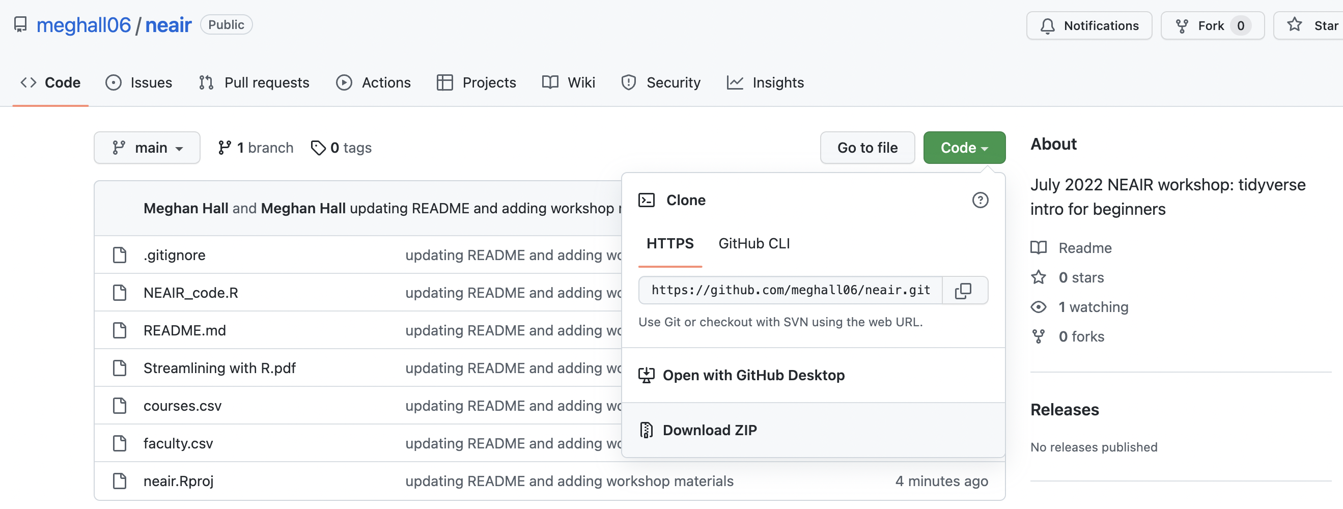
click big green Code button and select “Download ZIP”, then open neair.Rproj
Accessing data
1 2 3 4 5 6
use read_csv() to import a csv file
the readxl package is helpful for Excel files
view the data with View(faculty) or by clicking on the data name in the Environment pane
More data manipulation
1 2 3 4 5 6
Stringr functions
1 2 3 4 5 6
functions from stringr (which all start with str_) are useful for working with text data
| year | id | rank | dept1 | dept2 |
|---|---|---|---|---|
| 2021-22 | 1022 | Professor | Physics | Engineering |
| 2021-22 | 1059 | Professor | Physics | |
| 2021-22 | 1086 | Assistant Professor | Music | |
| 2021-22 | 1118 | Assistant Professor | Sociology | |
| 2021-22 | 1158 | Assistant Professor | Political Science | |
| 2021-22 | 1161 | Assistant Professor | Sociology |
Stringr functions
1 2 3 4 5 6
cheat sheet of functions is here
Pivoting data
1 2 3 4 5 6
existing faculty data has one row per faculty, some with multiple departments (sometimes known as wide data)
| year | id | rank | dept1 | dept2 |
|---|---|---|---|---|
| 2021-22 | 1005 | Lecturer | Chemistry | |
| 2021-22 | 1022 | Professor | Physics | Engineering |
| 2021-22 | 1059 | Professor | Physics | |
| 2021-22 | 1079 | Lecturer | Music | |
| 2021-22 | 1086 | Assistant Professor | Music | |
| 2021-22 | 1095 | Adjunct Instructor | Sociology |
Pivoting data
1 2 3 4 5 6
what if you instead want one row per faculty per department? (sometimes known as long data)
| year | id | rank | dept_no | dept |
|---|---|---|---|---|
| 2021-22 | 1005 | Lecturer | dept1 | Chemistry |
| 2021-22 | 1022 | Professor | dept1 | Physics |
| 2021-22 | 1022 | Professor | dept2 | Engineering |
| 2021-22 | 1059 | Professor | dept1 | Physics |
| 2021-22 | 1079 | Lecturer | dept1 | Music |
| 2021-22 | 1086 | Assistant Professor | dept1 | Music |
Pivoting data
1 2 3 4 5 6
the pivot_longer function lengthens data
Pivoting data
1 2 3 4 5 6
and pivot_wider does the opposite!
| semester | course_id | faculty_id | dept | enrollment | level |
|---|---|---|---|---|---|
| 20212202 | 10605 | 1772 | Physics | 7 | UG |
| 20212202 | 10605 | 1772 | Physics | 32 | GR |
Joining data
1 2 3 4 5 6
R has many useful functions for handling relational data
all you need is at least one key variable that connects data sets
left_join is most common, but there are more
Joining data
1 2 3 4 5 6
what’s the average UG enrollment per year, per faculty rank?
faculty
| year | id | rank | dept1 | dept2 |
|---|---|---|---|---|
| 2021-22 | 1005 | Lecturer | Chemistry | |
| 2021-22 | 1022 | Professor | Physics | Engineering |
| 2021-22 | 1059 | Professor | Physics | |
| 2021-22 | 1079 | Lecturer | Music |
courses
| semester | course_id | faculty_id | dept | enrollment | level |
|---|---|---|---|---|---|
| 20212202 | 10605 | 1772 | Physics | 7 | UG |
| 20212202 | 10605 | 1772 | Physics | 32 | GR |
| 20212202 | 11426 | 1820 | Political Science | 8 | UG |
| 20212202 | 12048 | 1914 | English | 24 | UG |
faculty$id is the same as courses$faculty_id
Joining data
1 2 3 4 5 6
what’s the average UG enrollment per year, per faculty rank?
| semester | course_id | faculty_id | dept | enrollment | level |
|---|---|---|---|---|---|
| 20212202 | 10605 | 1772 | Physics | 7 | UG |
| 20212202 | 10605 | 1772 | Physics | 32 | GR |
| 20212202 | 11426 | 1820 | Political Science | 8 | UG |
| 20212202 | 12048 | 1914 | English | 24 | UG |
| 20212202 | 13269 | 1095 | Sociology | 48 | UG |
- filter to
UGcourses only - create our
yearvariable again - summarize
enrollmentbyyearandfaculty_id
Joining data
1 2 3 4 5 6
use the <- operator to create a new data frame courses_UG
Joining data
1 2 3 4 5 6
filter to undergraduate courses only and mutate a new academic year variable
Joining data
1 2 3 4 5 6
group_by year and faculty member; summarize enrollment
| year | faculty_id | enr |
|---|---|---|
| 2018-19 | 1059 | 35 |
| 2018-19 | 1086 | 14 |
| 2018-19 | 1102 | 37 |
| 2018-19 | 1203 | 25 |
Joining data
1 2 3 4 5 6
what’s the average UG enrollment per year, per faculty rank?
faculty
| year | id | rank | dept1 | dept2 |
|---|---|---|---|---|
| 2021-22 | 1005 | Lecturer | Chemistry | |
| 2021-22 | 1022 | Professor | Physics | Engineering |
| 2021-22 | 1059 | Professor | Physics | |
| 2021-22 | 1079 | Lecturer | Music | |
| 2021-22 | 1086 | Assistant Professor | Music | |
| 2021-22 | 1095 | Adjunct Instructor | Sociology |
courses_UG
| year | faculty_id | enr |
|---|---|---|
| 2021-22 | 1005 | 50 |
| 2021-22 | 1086 | 17 |
| 2021-22 | 1095 | 48 |
| 2021-22 | 1128 | 32 |
| 2021-22 | 1147 | 32 |
| 2021-22 | 1191 | 7 |
Joining data
1 2 3 4 5 6
1
2
3
- new data frame
- data frame you’re adding data to
- data frame where the new data is coming from
| year | id | rank | dept1 | dept2 | enr |
|---|---|---|---|---|---|
| 2021-22 | 1005 | Lecturer | Chemistry | 50 | |
| 2021-22 | 1022 | Professor | Physics | Engineering | |
| 2021-22 | 1059 | Professor | Physics | ||
| 2021-22 | 1079 | Lecturer | Music | ||
| 2021-22 | 1086 | Assistant Professor | Music | 17 | |
| 2021-22 | 1095 | Adjunct Instructor | Sociology | 48 |
Joining data
1 2 3 4 5 6
what’s the average UG enrollment per year, per faculty rank?
| year | rank | avg_enr |
|---|---|---|
| 2021-22 | Adjunct Instructor | 34.66667 |
| 2021-22 | Assistant Professor | 23.60000 |
| 2021-22 | Associate Professor | 17.25000 |
| 2021-22 | Lecturer | 31.83333 |
| 2021-22 | Professor | 32.16667 |
| 2021-22 | Visiting Researcher |
Data visualization
1 2 3 4 5 6
ggplot2
1 2 3 4 5 6
ggplot2 is the data visualization package that is loaded with the tidyverse
the grammar of graphics maps data to the aesthetic attributes of geometric points
encoding data into visual cues (e.g., length, color, position, size) is how we signify changes and comparisons
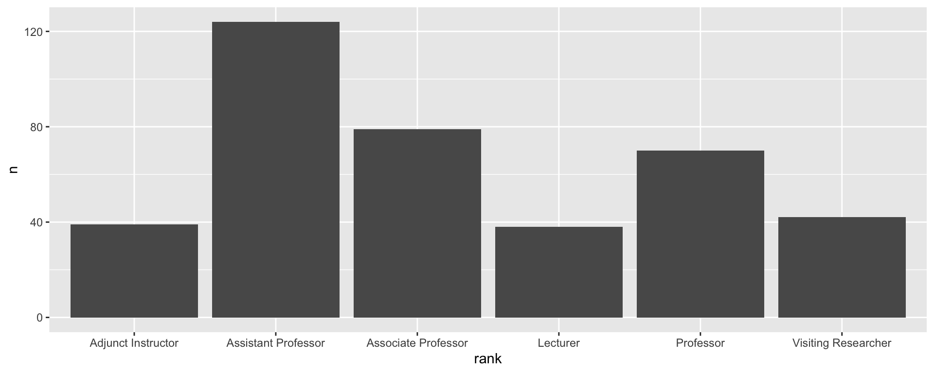
Bar chart
1 2 3 4 5 6
to combine lines into one code chunk, use + instead of %>%
Bar chart
1 2 3 4 5 6
can create a prettier plot pretty easily
expand for full code
faculty %>%
  count(rank) %>%
  ggplot(aes(x = reorder(rank, -n), y = n)) +
  geom_bar(stat = "identity", fill = "#cc0000") +
  scale_y_continuous(expand = expansion(mult = c(0, 0.1))) +
  geom_text(aes(label = n), vjust = -0.5) +
  labs(x = NULL, y = NULL,
       title = "Count of faculty by rank, 2018-2021") +
  theme_linedraw() +
  theme(panel.grid.major.x = element_blank(),
        axis.ticks = element_blank())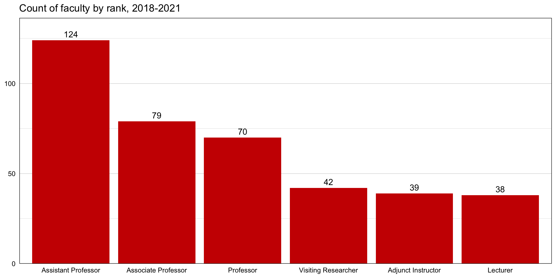
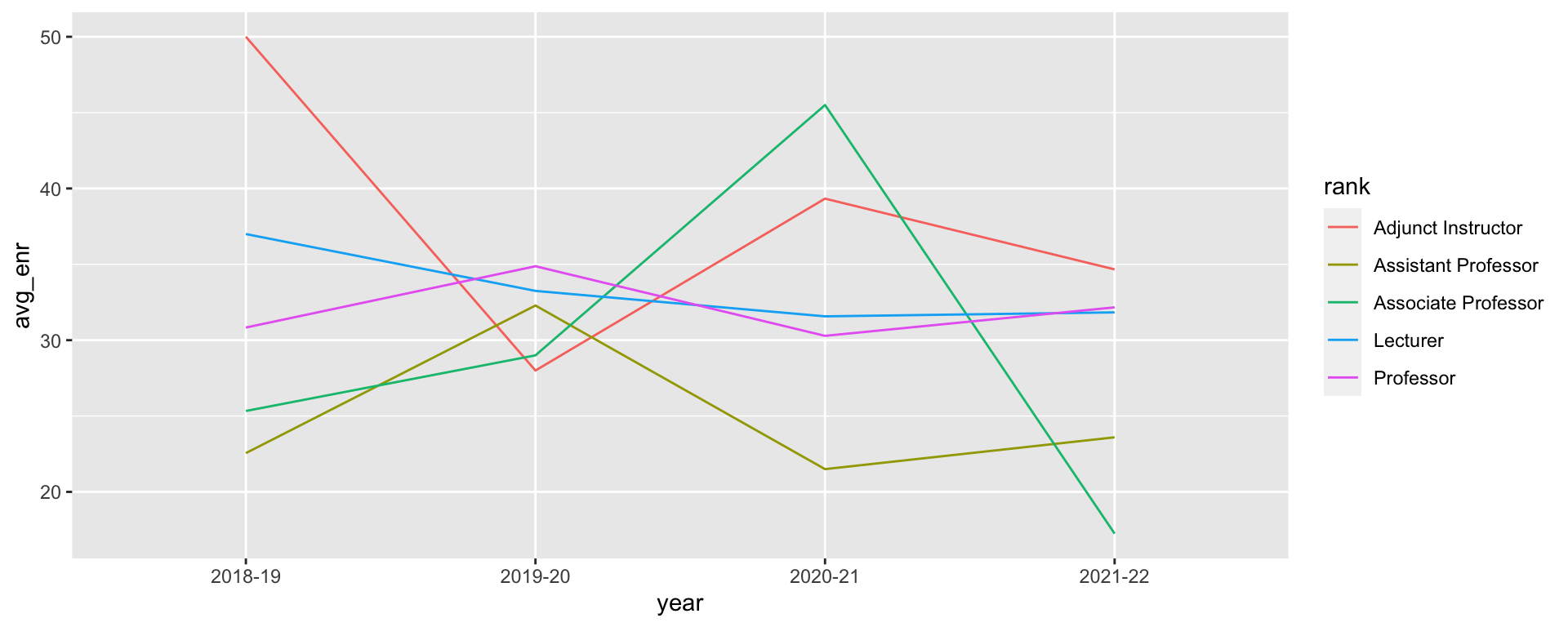
Line graph
1 2 3 4 5 6
Line graph
1 2 3 4 5 6
expand for full code
fac_enr %>%
  filter(!is.na(avg_enr)) %>%
  ggplot(aes(x = year, y = avg_enr, group = rank, color = rank)) +
geom_line() +
geom_point() +
scale_color_brewer(type = "qual", palette = "Dark2") +
labs(x = NULL, y = "Average enrollment",
title = "Average undergraduate enrollment per rank over time") +
theme_linedraw() +
theme(panel.grid.major.x = element_blank(),
axis.ticks = element_blank(),
legend.title = element_blank(),
legend.background = element_rect(fill = NA),
legend.key = element_rect(fill = NA),
legend.position = c(0.85, 0.82))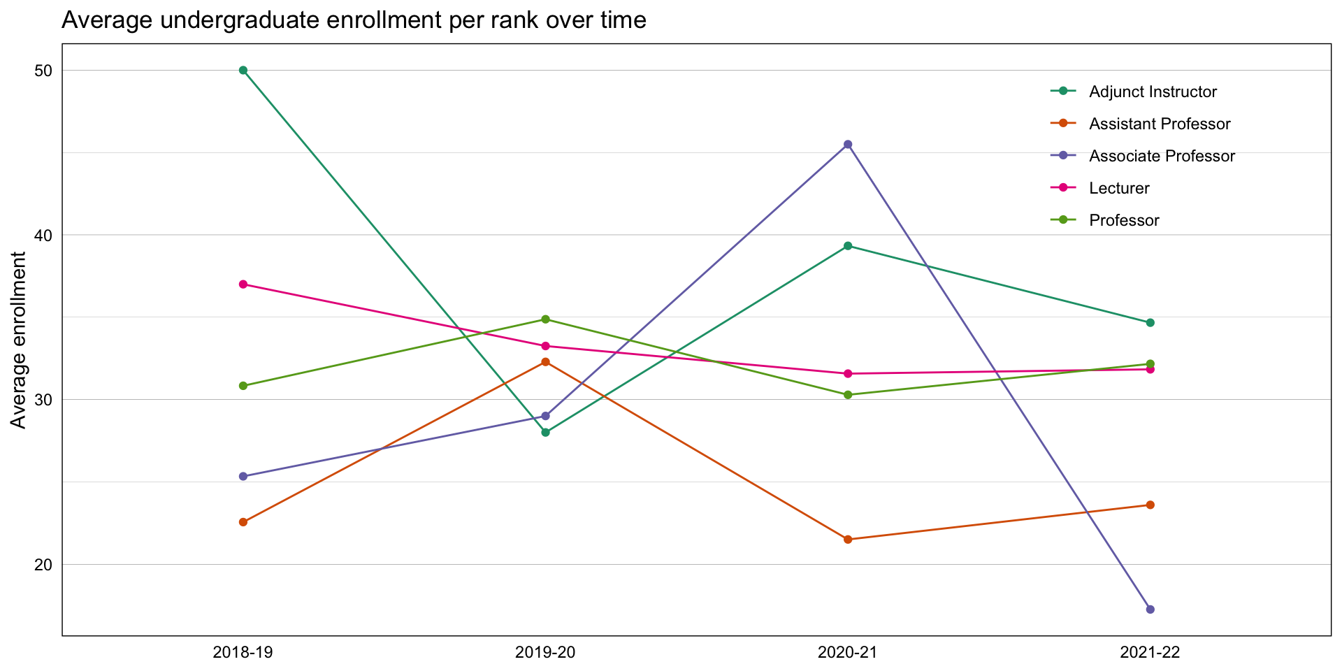
ggplot2 resources
1 2 3 4 5 6
from R for Data Science
Data Visualization: a practical introduction
creating custom themes
the ggplot2 book
the R graph gallery
Putting it all together
1 2 3 4 5 6
with what we’ve done so far, your .R file could:
- import your data files
- document all data cleaning and preparation steps and decisions
- produce a PPT-ready graphic summarizing your results
and that file would make it extremely easy for you or someone else to reproduce this analysis with new data in six months
Advanced topics
1 2 3 4 5 6
R Markdown
1 2 3 4 5 6
using RStudio, create .Rmd documents that combine text, code, and graphics
many output formats: html, pdf, Word, slides
exceedingly useful for parameterized reporting: can create an R-based PDF report and generate it automatically for, say, each department
Internal packages
1 2 3 4 5 6
you can also create your own packages!
your package can hold:
- common data sets that are used across projects
- custom
ggplot2themes - common functions and calculations (and their definitions!)
can be stored on a shared drive to facilitate collaboration
R Markdown and package resources
1 2 3 4 5 6
R Markdown
the official R Markdown website
R Markdown: The Definitive Guide
internal packages
a comprehensive theoretical explainer
a talk I gave earlier this year on the topic
Learn more about R
Resources
R for Data Science: the ultimate guide
R for Excel users: a very useful workshop
STAT 545: an online book on reproducible data analysis in R
the RStudio Education site
the Learn tidyverse site